Introduction

Click here to download the atlas

The pigeon brain atlas is a 3-dimensional model of the pigeon brain, constructed from several MRI and CT imaging sequences. Detailed information about the construction of the atlas and the acquired datasets can be found in our accompanying publication:
Gunturkun O., Verhoye M., De Groof G., Van der Linden A. (2012). A 3-Dimensional Digital Atlas of the Ascending Sensory and the Descending Motor Systems in the Pigeon Brain. Brain Struct Funct. 2013 Jan;218(1):269-81. doi: 10.1007/s00429-012-0400-y. Epub 2012 Feb 25.

In total, the pigeon brain atlas consists of 3 co-registered raw MRI and CT datasets and 6 brain delineation sets that can be downloaded freely. All brain delineation sets and the 3 co-registered MRI and CT datasets have been constructed in the same reference frame, and thus can be interchanged or superimposed at will without losing stereotactic information.

Below we will describe some basic features of two common 3D visualization packages (MRIcro and ImageJ), and how these programs can be used to visualize, modify and customize the datasets to fit your own ends. Of course, if you are familiar with other visualization software it is always better to use your preferred programs instead. To this end, all datasets are stored in a common file format for 3D datasets (Analyze 7.5), but if your software package does not support this file format, feel free to contact us and we will gladly provide you with a convenient file format.

The delineation sets are highly informative and very useful if you are not so well-known with the bird brain or if you simply want to know the stereotactic location of a delineated structure. Nevertheless, the information in these delineation sets is limited and inevitable biased to our own impressions. Therefore, we would like to encourage you to take the time to explore the raw datasets when possible, and discover the wealth of information that can be found in them. Even if your region of interest has been overlooked by us, with the right anatomical knowledge chances are high that you can still locate your ROI in one or more of the raw datasets, and customize the atlas to your advantage.

The brain atlas presented here is easy to adjust and we are always open to suggestions to make the atlas more informative and more useful to different scientific disciplines.

The default data orientation is presented in a similar fashion as previously published atlases, with a head-angle of 45 degrees. The 45º angle has been calculated based on the axis through the earcanal (the most likely position for fixating earbars) and the most posterior end of the beak opening relative to the horizontal plane. When loaded into MRIcro, the stereotactic zero point according to the Karten and Hodos pigeon atlas (1967) is reset to the zero-coordinate by default. This reference-point can be manually altered however, if another zero-coordinate is preferred. In this reference frame, the X-axis represents the brains left-to-right axis, the Y-axis corresponds to the posterior-anterior axis, and the Z-axis corresponds to the dorsal-ventral axis of the brain. The stereotactic coordinates of a specific brain area can be easily acquired by moving the cursor onto the desired region.

All datasets are provided in Analyze format, which is a common file format that can be read by most 3D visualization software packages. Analyze datasets always consist of two files, one file containing the raw data (*.img) and one file containing the header information, including the stereotactic coordinate settings (*.hdr). To function properly, both files must be present in the same folder.

Two software packages that are particularly suited to visualize the atlas datasets are MRIcro and ImageJ. Here we will describe some basic functions and useful options of MRIcro when working with the datasets. For more detailed information about both programs, we would like to refer you to the corresponding websites.

MRIcro: Opening and visualizing the datasets
To open a dataset, select “Open image…[Analyse or VoxBo]” under the [File] menu (or press Ctrl+O), and select the *.hdr file of the dataset you wish to view (e.g. T2.hdr).

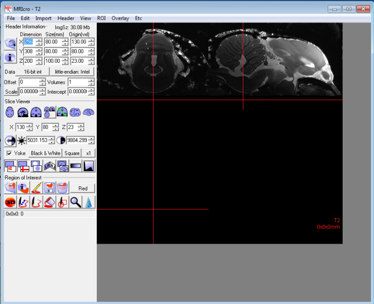
The ‘header information’ (top left) will show the dimensions of the data file (X,Y,Z), the size of each voxel, and the voxel position of the origin (this is the voxel position corresponding with 0,0,0 in the coordinate system). Note that the voxel size should be read as µm where it says mm (more on this later).

The ‘slice viewer’ (middle left) will show the sectioning plane through the dataset (which on first load is the horizontal plane through the origin), and allows you to change the section, plane, contrast/brightness, and show/hide crossbar information.

The ‘region of interest’ module (bottom left) shows the cursor position information and contains several selection tools.

T2 image data in MRIcro projection view. Crossbars correspond to the X,Y,Z values selected in the Slice Viewer module and coordinate information (shown in the bottom right of the display window) is relative to the origin. Both can be displayed by selecting the appropriate buttons in the Slice Viewer module.

MRIcro: Reading out coordinates

All coordinates displayed in MRIcro are relative to the origin voxel, selected in the header. MRIcro has originally been build for human brain data, and therefore the minimum unit is in millimeters. Unfortunately this cannot be modified, and therefore we have scaled up the birdbrain data by a factor 1000, to increase coordinate accuracy. Thus, where coordinates are displayed in mm, one has to read these coordinates in µm.

The simplest way to read out the coordinates of a specific area is by moving the mouse pointer over the area of interest in de data window. The information panel on the bottom of the ‘Region of interest’ module then indicates the XxYxZ coordinate (in µm) corresponding with the position of the mouse pointer followed by the grey value of the selected voxel. The X-coordinate is negative for the left, and positive for the right hemisphere; the Y-coordinate is positive anterior to the zero-point, and negative posterior of zero; the Z-coordinate is positive above zero, and negative below the zero-point.

Alternatively, one can choose to display the crossbar and coordinate information by selecting the appropriate buttons in the ‘Slice Viewer’ module. Crossbars shown in the data window, represent the sectioning planes, and the center of the crossbars correspond with the X,Y,Z values selected in the ‘Slice Viewer’ module. The coordinates of the crossbar center (in µm) can then be found at the bottom right of the data window.

MRIcro: Superimposing multiple datasets

All datasets can be superimposed with up to two other datasets (e.g. MRI brain data overlaying CT skull data) or delineation sets (e.g. Brain Nuclei and Fiber tracts overlaying MRI brain data). To do so, open a dataset (e.g. T2.hdr); then select “load image overlay” under the [Overlay] menu, and select the desired overlay file (e.g. auditory1.hdr).

Each delineated area corresponds with an indexed number, or grey value. This number can be found in the information panel of the ‘region of interest’ module (integer value between brackets). The legend for each delineation set can be found in the Data Description section below. If two delineation sets are superimposed on an MRI dataset, one delineation set has to be attributed ‘positive’ values and one set has to be given ‘negative’ values. Index numbers of delineated areas in the ‘negative’ group still correspond to the legend, excluding the ‘minus’ sign.

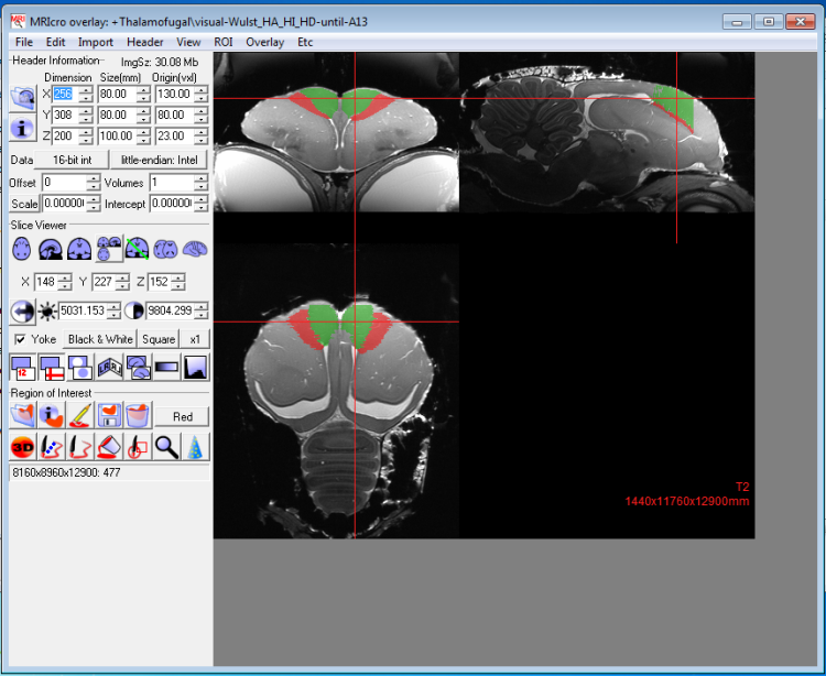
Superimposed images can be attributed different color schemes and transparency effects to optimize the visibility of different structures. Where each delineated region can be displayed with different colors, the index number of each region remains the same, and thus the legend remains unaltered.

T2 image data with superimposed visual Wulst. Crossbar indicates the Hyperpallium apicale, corresponding with index number 1 (shown as integer between [#] in the information panel when hovered over with mouse). Coordinates of this region can be found in the information panel and on the bottom right of the data window.